Proximal Algorithms in Federated Learning

In non-I.I.D. scenarios, based on the idea of reducing the impact of local updates of clients on the global model, [Li et al.[1]] first introduced a proximal term to the local objective functions, aiming at making the algorithm more stable and converging faster. Compared to SCAFFOLD, methods using proximal terms do not need to maintain extra parameters (mainly related to the gradients), hence having no communication overhead and no additional cost to security (refer to [Zhu et al.[2]] for more details).

To be more specific, in the \((t+1)\)-th iteration, the local objective function of client \(k\) changes from \(f_k(\theta_k)\) to the following form with a proximal term:

(1)\[ \begin{align}\begin{aligned}\DeclareMathOperator*{\expectation}{\mathbb{E}} \DeclareMathOperator*{\minimize}{minimize} \newcommand{\R}{\mathbb{R}}\\h_k(\theta_k, \theta^{(t)}) := f_k(\theta_k) + \frac{\mu}{2} \lVert \theta_k - \theta^{(t)} \rVert^2,\end{aligned}\end{align} \]

where \(\mu\) is a penalty constant. It should be noticed that the proximal center \(\theta^{(t)}\) is the model parameter on the server node obtained in the previous iteration (the \(t\)-th iteration). Indeed, the overall optimization problem can be modeled as the following constrained optimization problem

(2)\[\begin{split}\begin{array}{cl} \minimize & \frac{1}{K} \sum\limits_{k=1}^K \left\{ f_k(\theta_k) + \frac{\mu}{2} \lVert \theta_k - \theta \rVert^2 \right\} \\ \text{subject to} & \theta = \frac{1}{K} \sum\limits_{k=1}^K \theta_k. \end{array}\end{split}\]

For alternatives for the proximal center, studies were conducted in [Hanzely and Richtárik[3], Li et al.[4]] which would be introduced later. Now, we summarize the pseudocode for FedProx as follows:

\begin{algorithm}
\caption{PseudoCode for \texttt{FedProx}}
\begin{algorithmic}
\REQUIRE penalty constant $\mu,$ constant $\gamma \in [0, 1]$

\STATE {Initiation:}
\STATE global model parameters $\theta^{(0)} \in \mathbb{R}^d$

\FOR{each round $t = 0, 1, \cdots, T-1$}
\STATE $\mathcal{S}^{(t)} \gets$ (random set of clients) $\subseteq [K]$
\STATE broadcast $\theta^{(t)}$ to clients $k \in \mathcal{S}^{(t)}$
\STATE \FOR{each client $k \in \mathcal{S}^{(t)}$ {in parallel}}
\STATE find a $\gamma$-inexact solution $\theta_k^{(t)}$ to $\underset{\theta_k}{\text{argmin}} h_k(\theta_k, \theta^{(t)}) := f_k(\theta_k) + \frac{\mu}{2} \lVert \theta_k - \theta^{(t)} \rVert^2$
\STATE \COMMENT{Definition of $\gamma$-inexactness: $\nabla h_k(\theta_k^*, \theta^{(t)}) \leqslant \gamma h_k(\theta_k, \theta^{(t)}),$ where $\theta_k^*$ is the exact solution to $h_k.$}
\STATE send $\theta_k^{(t)}$ to server
\STATE \ENDFOR

\STATE {Server Update:}
\STATE $\hspace{1.3em}$ $\theta^{(t+1)} \gets \frac{1}{\lvert \mathcal{S}^{(t)} \rvert} \sum\limits_{k\in \mathcal{S}^{(t)}} \theta_k^{(t)}$
\ENDFOR
\end{algorithmic}
\end{algorithm}

We denote the \(\gamma\)-inexact solution \(\theta_k^{(t)}\) as

(3)\[ \begin{align}\begin{aligned}\DeclareMathOperator*{\argmax}{arg\,max} \DeclareMathOperator*{\argmin}{arg\,min} % \DeclareMathOperator*{\prox}{prox} \newcommand{\prox}{\mathbf{prox}}\\\theta_k^{(t)} \approx \prox_{f_k, \mu} (\theta^{(t)}) := \argmin\limits_{\theta_k} \left\{ f_k(\theta_k) + \frac{\mu}{2} \lVert \theta_k - \theta^{(t)} \rVert^2 \right\},\end{aligned}\end{align} \]

where \(\prox_{f_k, \mu}\) is the proximal operator [Moreau[5]] of \(f_k\) with respect to \(\mu\). Let \(s = \frac{1}{\mu}\), since one has \(\prox_{f_k, \mu} = \prox_{sf_k, 1}\), we also denote \(\prox_{f_k, \mu}\) as \(\prox_{sf_k}\). Corresponding function

(4)\[\mathcal{M}_{sf_k} (\theta^{(t)}) = \mathcal{M}_{f_k, \mu} (\theta^{(t)}) := \inf\limits_{\theta_k} \left\{ f_k(\theta_k) + \frac{\mu}{2} \lVert \theta_k - \theta^{(t)} \rVert^2 \right\}\]

is called Moreau envelope or Moreau-Yosida regularization of \(f_k\) with respect to \(\mu\). Moreau envelope of a function \(f_k\) has the following relationship [Parikh and Boyd[6]] with its proximal operator:

(5)\[\prox_{sf_k} (\theta) = \theta - s \nabla \mathcal{M}_{sf_k} (\theta), ~ \forall \theta \in \R^d.\]

Namely, \(\prox_{sf_k}\) can be regarded as the gradient descent operator for minimizing \(\mathcal{M}_{sf_k}\) with step size \(s\).

For the convergence of FedProx in non-I.I.D. scenarios, [Li et al.[1]] has the following theorem:

Theorem ([Li et al.[1]] Theorem 4)

Assume that the objective functions on clients \(\{f_k\}_{k=1}^K\) are non-convex, \(L\)-smooth (definition see (3)), and there exists a constant \(L_- > 0\) such that \(\nabla^2 f_k \succcurlyeq -L_- I_d\). Assume further that the functions \(\{f_k\}_{k=1}^K\) satisfy the so-called bounded dissimilarity condition, i.e. for any \(\varepsilon > 0\), there exists a constant \(B_{\varepsilon} > 0\) such that for any point \(\theta\) in the set \(\mathcal{S}_{\varepsilon}^c := \{ \theta ~|~ \lVert \nabla f(\theta) \rVert^2 > \varepsilon\}\), the following inequality holds

(6)\[B(\theta) := \frac{\expectation_k [\lVert \nabla f_k(\theta) \rVert^2]}{\lVert \nabla f(\theta) \rVert^2} \leqslant B_{\varepsilon}.\]

Fix constants \(\mu, \gamma\) satisfying

(7)\[\rho := \left( \frac{1}{\mu} - \frac{\gamma B}{\mu} - \frac{B(1+\gamma)\sqrt{2}}{\bar{\mu}\sqrt{K}} - \frac{LB(1+\gamma)}{\bar{\mu}\mu} - \frac{LB^2(1+\gamma)^2}{2\bar{\mu}^2} - \frac{LB^2(1+\gamma)^2}{\bar{\mu}^2 K} \left( 2\sqrt{2K} + 2 \right) \right) > 0,\]

where \(\bar{\mu} = \mu - L_- > 0\). Then, in the \((t+1)\)-th iteration of FedProx, assuming that the global model \(\theta^{(t)}\) of the previous iteration is not the first-order stationary point of the global objective function \(f(\theta)\), (i.e. \(\theta^{(t)} \in \mathcal{S}_{\varepsilon}^c\)), the following decrease in the global objective function holds

(8)\[\expectation\nolimits_{\mathcal{S}^{(t)}}[f(\theta^{(t+1)})] \leqslant f(\theta^{(t)}) - \rho \lVert \nabla f (\theta^{(t)}) \rVert^2.\]

Remark

For the convergence theorem of FedProx, we have the following observations: in a neighbourhood of some zero of \(\lVert \nabla f \rVert\), if this zero is not cancelled by \(\mathbb{E}_k[\lVert \nabla f_k \rVert]\), i.e. this point is also a zero of \(\mathbb{E}_k[\lVert \nabla f_k \rVert]\) with the same or higher multiplicity, then in the neighbourhood, \(B_{\varepsilon}\) goes rapidly to infinity as \(\varepsilon \to 0\), thus violating the condition \(\rho > 0\). In this case, the inequality (8) becomes meaningless.

When the data distribution across clients is identical (ideal case), then \(B_{\varepsilon}\) is constantly equal to 1, which would not have the problem mentioned above. This problem is the start point of a series of follow-up works [Pathak and Wainwright[7], Tran-Dinh et al.[8]].

The positive significance of the FedProx algorithm is that it first introduced the proximal point algorithms (PPA) in the field of federated learning, although which were only used for solving local optimization problems (or equivalently the inner loop problem) and the whole of the FedProx algorithm is not a PPA in strict sense. The FedProx algorithm provides not only a good framework for theoretical analysis, but also a good starting point for the design of new algorithms. A large proportion of the algorithms proposed later for personalized fedrated learning [Hanzely and Richtárik[3], Acar et al.[9], Li et al.[4], Dinh et al.[10], Li et al.[11]] rely on the proximal terms (or similar terms) as the main technical tool for personalization.

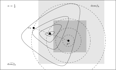
Schematic diagram for \(f_k(\alpha_k \omega_k + (1 - \alpha_k) \theta^*)\) in the APFL algorithm.

\begin{algorithm}
\caption{PseudoCode for \texttt{APFL}}
\begin{algorithmic}
\REQUIRE mixture weights $\alpha_1, \ldots, \alpha_K,$ synchronization gap $\tau$

\STATE {Initiation:}
    \STATE $\hspace{1.3em}$ {Init server:} global model parameters $\theta^{(0)} \in \mathbb{R}^d,$ random set of clients $S^{(t)} \subseteq [K]$
    \STATE $\hspace{1.3em}$ {Init clients:} local model parameters $\omega_k^{(0)} \in \mathbb{R}^d, ~ \theta_k^{(0)} \gets \theta^{(0)}, ~ \forall k \in [K]$
    \STATE $\hspace{1.3em}$ {Constants:} condition number $\kappa \gets \frac{L}{\mu},$ $a \gets \max\{128\kappa, \tau\}$

\FOR{each round $t = 0, 1, \cdots, T-1$}
    \FOR{each client $k \in \mathcal{S}^{(t)}$ {in parallel}}
        \STATE $\bar{\omega}_k^{(t)} \gets \alpha_k \omega_k^{(t)} + (1-\alpha_k) \theta_k^{(t)}$ \COMMENT{mixture model}
        \STATE $\eta^{(t)} \gets \frac{16}{\mu(t+a)}$ \COMMENT{decay learning rate}
        \STATE $\theta_k^{(t+1)} \gets \theta_k^{(t)} - \eta^{(t)} \nabla f_k(\theta_k^{(t)})$ \COMMENT{inner problem (global model) update}
        \STATE $\omega_k^{(t+1)} \gets \omega_k^{(t)} - \eta^{(t)} \nabla f_k(\bar{\omega}_k^{(t)})$ \COMMENT{outer problem (personalized model) update}
        \COMMENT{Optional: adaptive mixture weights update}
        \COMMENT{$\alpha_k \gets \alpha_k - \eta^{(t)} \nabla_{\alpha_k} f_k(\bar{\omega}_k^{(t)}) = \alpha_k - \eta^{(t)} \left\langle \omega_k^{(t)} - \theta_k^{(t)}, \nabla f_k(\bar{\omega}_k^{(t)}) \right\rangle$}
    \ENDFOR

    \IF{$t$ not divides synchronization gap $\tau$}
        \STATE {Server updates:} $\mathcal{S}^{(t+1)} \gets \mathcal{S}^{(t)}$
    \ELSE
        \STATE each client $k \in \mathcal{S}^{(t)}$ sends $\theta_k^{(t+1)}$ to server
        \STATE {Server updates:}
            \STATE $\hspace{1.3em}$ $\theta^{(t+1)} \gets \frac{1}{\# \mathcal{S}^{(t)}} \sum_{k \in \mathcal{S}^{(t)}} \theta_k^{(t+1)}$
            \STATE $\hspace{1.3em}$ $\mathcal{S}^{(t+1)} \gets$ (random set of clients) $\subseteq [K]$
            \STATE $\hspace{1.3em}$ broadcast $\theta^{(t+1)}$ to clients $k \in S^{(t+1)}:$ $\theta_k^{(t+1)} \gets \theta^{(t+1)}$
    \ENDIF
\ENDFOR

\STATE final personalized model: $\hat{\omega}_k \gets \frac{1}{S_T}\sum\limits_{t=1}^{T} p_t \left( \alpha_k \omega_k^{(t)} + (1-\alpha_k)\frac{1}{\#\mathcal{S}^{(t-1)}}\sum\limits_{k\in\mathcal{S}^{(t-1)}}\theta_k^{(t)} \right)$
\STATE final global model: $\hat{\theta} \gets \frac{1}{S_T}\sum\limits_{t=1}^{T} \frac{p_t}{\#\mathcal{S}^{(t-1)}} \sum\limits_{k\in\mathcal{S}^{(t-1)}}\theta_k^{(t)}$
\STATE where $p_t = (t+a)^2, S_T = \sum\limits_{t=1}^{T}p_t$
\end{algorithmic}
\end{algorithm}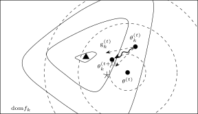

Client model parameter update schematic diagram of the FedDyn algorithm.

\begin{algorithm}
\caption{PseudoCode for \texttt{FedDyn}}
\begin{algorithmic}
\REQUIRE penalty coeffecient $\mu$

\STATE {\bfseries Initiation:}
\STATE $\hspace{1.3em}$ {\bfseries Init server:} global model parameters $\theta^{(0)} \in \mathbb{R}^d,$ $h = 0 \in \mathbb{R}^d$
\STATE $\hspace{1.3em}$ {\bfseries Init clients:} local gradient $\mathfrak{g}_k^{(0)} \gets 0 \in \mathbb{R}^d, ~ \forall k \in [K]$

\FOR{each round $t = 0, 1, \cdots, T-1$}
    \STATE $\mathcal{S}^{(t)} \gets$ (random set of clients) $\subseteq [K]$
    \STATE broadcast $\theta^{(t)}$ to clients $k \in \mathcal{S}^{(t)}$
    \FOR{each client $k \in \mathcal{S}^{(t)}$ {\bfseries in parallel}}
        \STATE $\theta_k^{(t+1)} \gets \underset{\theta_k}{\text{argmin}} \left\{ f_k(\theta_k) - \langle \mathfrak{g}_k^{(t)}, \theta_k \rangle + \frac{\mu}{2} \lVert \theta_k - \theta^{(t)} \rVert^2 \right\}$
        \STATE $\mathfrak{g}_k^{(t+1)} \gets \mathfrak{g}_k^{(t)} - \mu (\theta_k^{(t+1)} - \theta^{(t)})$ \COMMENT{update local gradient}
        \STATE send $\theta_k^{(t+1)}$ to server
    \ENDFOR
    \STATE {\bfseries Server Update:}
    \STATE $\hspace{1.3em}$ $h^{(t+1)} \gets h^{(t)} - \frac{\mu}{K} \left(\sum\limits_{k \in \mathcal{S}^{(t)}} \theta_k^{(t+1)} - \theta^{(t)} \right)$
    \STATE $\hspace{1.3em}$ $\theta^{(t+1)} \gets \left( \frac{1}{\# \mathcal{S}^{(t)}}\sum\limits_{k \in \mathcal{S}^{(t)}} \theta_k^{(t+1)} \right) - \frac{1}{\mu} h^{(t+1)}$
\ENDFOR
\end{algorithmic}
\end{algorithm}

FedDC: Federated Learning with Local Drift Decoupling and Correction

The proximal term of FedProx pulls each local model towards the global one, tacitly treating the gap between them as a nuisance to be suppressed. Under statistical heterogeneity, however, a nonzero drift between the local and the global model is inherent rather than incidental: the local models should deviate from the global one to better fit their own data distributions. The federated learning algorithm with local drift decoupling and correction (FedDC, see arXiv:2203.11751) therefore decouples the local drift into an auxiliary variable \(h_i\) maintained by client \(i\), which tracks the gap between its local model and the global one. The ideal restriction \(h_i = w - \theta_i\) is relaxed into a penalized term, and the local objective of client \(i\) in round \(t\) reads

(9)\[F(\theta_i; h_i, D_i, w) = L_i(\theta_i) + \frac{\alpha}{2} \left\lVert \theta_i + h_i - w \right\rVert^2 + \frac{1}{\eta K} \langle \theta_i, g_i - g \rangle,\]

where \(L_i\) is the empirical loss on \(D_i\), \(\alpha > 0\) weights the parameter correction term, \(\eta\) is the learning rate, \(K\) is the number of local iterations per round, and \(g_i\) (resp. \(g\)) denotes the last local update value \(g_i = \theta_i^{+} - \theta_i\) (resp. its sample-size weighted average \(g = \sum_{i=1}^N \frac{\lvert D_i \rvert}{\lvert D \rvert} g_i\)); the inner-product term, adopted from SCAFFOLD [Karimireddy et al.[12]], corrects the gradient drift. Note that the center of the quadratic term is \(w - h_i\), i.e. the proximal center of FedProx corrected by the drift.

Each round, client \(i\) initializes \(\theta_i = w\) and performs \(K\) local gradient steps on \(F\), which in closed form amounts to

(10)\[\theta_i^{k+1} = \theta_i^{k} - \eta \nabla L_i(\theta_i^{k}) - \eta \alpha \left( \theta_i^{k} + h_i - w \right) - \frac{1}{K} \left( g_i - g \right).\]

Afterwards, the drift variable is updated reusing the local update (so that no additional backpropagation is needed),

(11)\[h_i^{+} = h_i + \left( \theta_i^{+} - \theta_i \right),\]

and the drift-corrected local parameters \(\theta_i^{+} + h_i^{+}\) are uploaded, of which the server takes the sample-size weighted average as the new global model,

(12)\[w^{+} = \sum_{i=1}^N \frac{\lvert D_i \rvert}{\lvert D \rvert} \left( \theta_i^{+} + h_i^{+} \right).\]

The pseudocode is summarized below.

\begin{algorithm}
\caption{PseudoCode for \texttt{FedDC}}
\begin{algorithmic}
\REQUIRE number of clients $N,$ number of rounds $T,$ local iterations $K,$ learning rate $\eta,$ correction coefficient $\alpha$

\STATE {Initiation:}
\STATE $w^0$ on the server
\STATE $\theta_i^0 = w^0$ and $h_i^0 = 0$ for all $i \in [N]$ on the clients

\FOR{each round $t = 0, 1, \cdots, T-1$}
\STATE the server downloads $w^t$ (and $g^t$, if any) to the clients
\STATE \FOR{each client $i$ {in parallel}}
\STATE $\theta_i^{t,0} = w^t$
\FOR{$k = 0, 1, \cdots, K-1$}
\STATE $\hspace{1.3em}$ $\theta_i^{t,k+1} = \theta_i^{t,k} - \eta \nabla L_i(\theta_i^{t,k}) - \eta \alpha \left( \theta_i^{t,k} + h_i^t - w^t \right) - \frac{1}{K} \left( g_i^t - g^t \right)$
\STATE \ENDFOR
\STATE $\theta_i^+ = \theta_i^{t,K}$
\STATE $h_i^{t+1} = h_i^t + \left( \theta_i^+ - w^t \right)$
\STATE $g_i^{t+1} = \theta_i^+ - w^t$
\STATE upload $\theta_i^+ + h_i^{t+1}$ and $g_i^{t+1}$ to the server
\STATE \ENDFOR
\STATE {Server Update:}
\STATE $w^{t+1} = \sum\limits_{i=1}^N \frac{\lvert D_i \rvert}{\lvert D \rvert} \left( \theta_i^+ + h_i^{t+1} \right)$
\STATE $g^{t+1} = \sum\limits_{i=1}^N \frac{\lvert D_i \rvert}{\lvert D \rvert} g_i^{t+1}$
\ENDFOR
\end{algorithmic}
\end{algorithm}

References

[1] (1,2,3)

Tian Li, Anit Kumar Sahu, Manzil Zaheer, Maziar Sanjabi, Ameet Talwalkar, and Virginia Smith. Federated Optimization in Heterogeneous Networks. In I. Dhillon, D. Papailiopoulos, and V. Sze, editors, Proceedings of Machine Learning and Systems, volume 2, 429–450. 2020.

[2]

Ligeng Zhu, Zhijian Liu, and Song Han. Deep Leakage from Gradients. Advances in Neural Information Processing Systems, 32:14774–14784, 2019.

[3] (1,2)

Filip Hanzely and Peter Richtárik. Federated Learning of a Mixture of Global and Local Models. arXiv preprint arXiv:2002.05516, 2020.

[4] (1,2)

Tian Li, Shengyuan Hu, Ahmad Beirami, and Virginia Smith. Ditto: Fair and Robust Federated Learning Through Personalization. In Marina Meila and Tong Zhang, editors, Proceedings of the 38th International Conference on Machine Learning, volume 139 of Proceedings of Machine Learning Research, 6357–6368. PMLR, 7 2021.

[5]

J.J. Moreau. Proximité et Dualité dans un Espace Hilbertien. Bulletin de la Société Mathématique de France, 79:273–299, 1965. doi:10.24033/bsmf.1625.

[6]

Neal Parikh and Stephen Boyd. Proximal Algorithms. Foundations and Trends® in Optimization, 1(3):127–239, 2014. doi:10.1561/2400000003.

[7]

Reese Pathak and Martin J Wainwright. FedSplit: An Algorithmic Framework for Fast Federated Optimization. In H. Larochelle, M. Ranzato, R. Hadsell, M.F. Balcan, and H. Lin, editors, Advances in Neural Information Processing Systems, volume 33, 7057–7066. Curran Associates, Inc., 2020.

[8]

Quoc Tran-Dinh, Nhan Pham, Dzung T. Phan, and Lam M. Nguyen. FedDR – Randomized Douglas-Rachford Splitting Algorithms for Nonconvex Federated Composite Optimization. In A. Beygelzimer, Y. Dauphin, P. Liang, and J. Wortman Vaughan, editors, Advances in Neural Information Processing Systems. 2021.

[9]

Durmus Alp Emre Acar, Yue Zhao, Ramon Matas, Matthew Mattina, Paul Whatmough, and Venkatesh Saligrama. Federated Learning Based on Dynamic Regularization. In International Conference on Learning Representations. 2021.

[10]

Canh T. Dinh, Nguyen H. Tran, and Tuan Dung Nguyen. Personalized Federated Learning with Moreau Envelopes. In Proceedings of the 34th International Conference on Neural Information Processing Systems. Red Hook, NY, USA, 2020. Curran Associates Inc.

[11]

Yinchuan Li, Xiaofeng Liu, Xu Zhang, Yunfeng Shao, Qing Wang, and Yanhui Geng. Personalized Federated Learning via Maximizing Correlation with Sparse and Hierarchical Extensions. arXiv preprint arXiv:2107.05330, 2021.

[12]

Sai Praneeth Karimireddy, Satyen Kale, Mehryar Mohri, Sashank Reddi, Sebastian Stich, and Ananda Theertha Suresh. SCAFFOLD: Stochastic Controlled Averaging for Federated Learning. In International Conference on Machine Learning, 5132–5143. PMLR, 2020.